
By Martin Jansen, Owner of Jansen-PCINFO
This article is for someone who is a beginner with spreadsheets, but instead of trying to just learn about rows and columns, we’ll learn about creating a useful monthly budget spreadsheet.
With inflation on the rise most of us need to control our spending, determining how best to use our money. In any budget there are necessary expenses that must be paid and then there are discretionary expenses where we can control our spending. We’ll try and define each type of spending in this article.
The software I am using for this article is LibreOffice Calc, but the principles can be applied to any spreadsheet program. LibreOffice is a suite of productivity applications that is cross-platform, available for Windows, macOS and Linux. Indeed, it is included as part of many distributions of Linux, like Linux Mint.
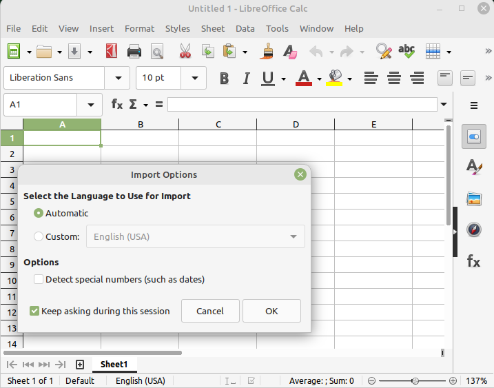
Let’s begin by opening LibreOffice Calc and typing in our heading in cell A1: Monthly Budget Worksheet. Or, you may copy and paste the heading text, clicking on OK for Import Options:
Don’t worry about how it looks right now, we’ll make it ‘pretty’ later. Type Month of: in A2 and in B2 we’ll type our first function: =TODAY() This will reveal today’s date. In C2 we’ll type another function: =TEXT(B2,”mmmm”) This extracts just the month text from the B2 formula.
In D2 type Total Income and in E2 type and estimate of your monthly income. Use round numbers like 6000. You’re probably more aware of your total monthly net income (take home pay) than any other expense numbers. If not, look at past paychecks and any other regular income for a given month.
In D3 type Income-Expense. Now skip down to A5 and type in Budget and in D5 type Actual. We’ll add functions or formulas a little later for E3, C5 and E5. Now, hold down the Ctrl key and press S (Ctrl+S) to save the document. Name the spreadsheet Budget.
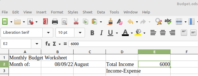
Our budget worksheet should look something like this now:
Here’s a list of common expense items along with brief description that can be used to copy and paste into A7 downward:
| Expenses | Explanation |
| Childcare | Taking care of your babies |
| Clothing | Kohl’s and other clothing stores |
| Debt Payments | Pay down credit cards and the like |
| Dining | Dining Out |
| Entertainment | Shows and Plays, Magazines, etc. |
| Groceries | Food and Beverages for the home |
| Housing | Rent or Mortgage Payments |
| Insurance | Life, Health, Property and Automobiles |
| Maintenance | Home Maintenance, fix or repair daily |
| Medical | Prescription and Doctor expenses |
| Miscellaneous | Any other small expenses |
| Personal Care | Haircuts, Stylists costs |
| Pets | Taking care of the fur babies |
| Savings | Set aside money for the future |
| Transportation | Car or public transportation costs |
| Utilities | Water, Gas, Electricity and Internet |
| Vacation | The cost of having fun |
Here’s an image of the same:
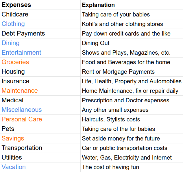
The blue represents categories where you can control spending, orange has some control and black, of course, are expenses that are not easily controlled.
Copy both columns and paste into A7, again OK on Import Options. Just the text carries over in the native font Liberation Serif. Moneydance, my favorite personal finance program, has a longer listing if the above expense categories don’t work for you. Delete or revise categories to your lifestyle.
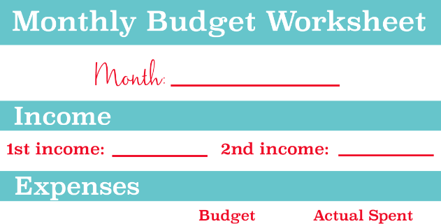
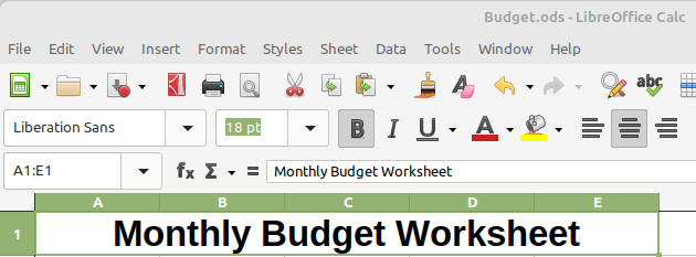
Now is the time to make things look a bit prettier. We’ll switch fonts from the default Liberation Serif to Liberation Sans (similar to Arial) and increase the font size. But first, use the mouse to drag from A1 to E1. This can also be done by selecting A1, pressing down the shift key and left arrowing over to E1. Next, we’ll click on the Format menu, click on Merge and Unmerge cells and select Merge and Center Cells. While the cells are still active, change the font to Liberation Sans and increase the size to 18 pt. Click on the B next to the font size (or Ctrl+B) to bold the text. The heading should now look like this:
While we’re changing fonts, let’s type Ctrl +A and switch to Liberation Sans for the whole worksheet.
Now select all of column A1 by clicking on the A in green. We’ll change the width of the column. This can be done by dragging the line between A and B or right clicking on A and setting the column width to 1.2” until the expense categories are listed without wrapping.
We’re going to hide column B since we don’t need to see the explanations of the categories or the =TODAY() formula. Place the cursor and right click on the B (in green) and select Hide Columns. The columns now go from A to C.
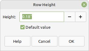
Because we pasted in the explanations the row height is now beyond the default size of .18”. We’ll select from 7 to the last listed expense item (for me, 24). Right click on row 7 (in green) and select the menu item Row Height. Put a checkmark in Default value and the rows will be set to .18”:
Now we will add our budget expense numbers for the month. This will require some research into what you are currently spending. It can be quite eye opening as you discover that you may be overspending on some items. Some people, for example, have a Starbucks or eating out habit that is inflating their Dining expense. It is much cheaper to make coffee and prepare meals at home, but not as convenient. I looked up some average monthly expenses and guessed on a few others:
| Expenses | |
| Childcare | 900 |
| Clothing | 100 |
| Debt Payments | 100 |
| Dining | 200 |
| Entertainment | 200 |
| Groceries | 800 |
| Housing | 1100 |
| Insurance | 500 |
| Maintenance | 200 |
| Medical | 100 |
| Miscellaneous | 50 |
| Personal Care | 100 |
| Pets | 50 |
| Savings | 200 |
| Transportation | 300 |
| Utilities | 500 |
| Vacation | 400 |
Try to be realistic about spending relative to your income, inputting the numbers that fit your lifestyle.
We’ve added a lot of data time to save (Ctrl+S) again.
We’ll now use the power of a spreadsheet to sum the budget numbers. Select the empty cell at the very bottom of the budget numbers. At the top of the spreadsheet next to the cell reference are the function wizards and shortcuts including the Sum function:
When I use the Sum function at the bottom of my list of budget numbers it automatically assumes that I want to add the numbers above, in my case above C25. The function now reads: =SUM(C8:C24), which totals 5800.
Now I will enter the actual spending numbers with less spending than budget in some categories and some overspending in others:
| Expenses | ||
| Childcare | 900 | 900 |
| Clothing | 100 | 75 |
| Debt Payments | 100 | 100 |
| Dining | 200 | 150 |
| Entertainment | 200 | 150 |
| Groceries | 800 | 900 |
| Housing | 1100 | 1100 |
| Insurance | 500 | 500 |
| Maintenance | 200 | 150 |
| Medical | 100 | 100 |
| Miscellaneous | 50 | 25 |
| Personal Care | 100 | 120 |
| Pets | 50 | 50 |
| Savings | 200 | 250 |
| Transportation | 300 | 300 |
| Utilities | 500 | 500 |
| Vacation | 400 | 500 |
For instance, my Groceries expenses are up because I purchased real beef steaks instead of tube steaks, i.e., hotdogs. With the actual values filled in, I can copy C25 and paste it into D25. The paste will add up the numbers in the D column, which is quicker than using the Sum function again, and will total 5870.
Now we use basic math to subtract the budget value of C8 from the actual value of D8. Select E8 and type in =D8-C8. Now copy and paste E8 into cells E9 though the end of the numbers in column D. The copy and paste works equally well for columns as well as rows of numbers as the function changes cells.
Finishing up now, I can Sum the additions and subtractions to see that I spent $70 over budget. I type the word Total in A25 right format and bolded it as well as the Sum functions at the bottom of the sheet. I put the word Difference in E7.
A little more math and we are done. In C5 and D5 I repeat the numbers in C25 and D25 typing in =C25 and =D25, respectively. In cell E3 I subtract my total income from my actual expenses: =E2-D25.
That’s it, our budget worksheet is complete. Now I can reuse it month to month, setting my budget at the beginning of the month and comparing actual expenses at the end of the month. I can even update the actual totals weekly to make sure I am on track. Here’s an image of my worksheet:
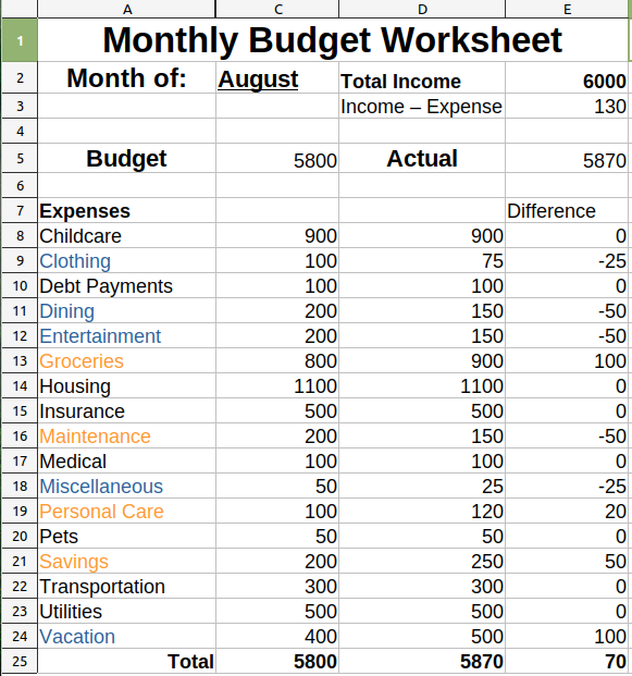
In building this worksheet, we hopefully learned something about spreadsheet basics along the way.